on
How to merge data from various sources in Google Sheets.
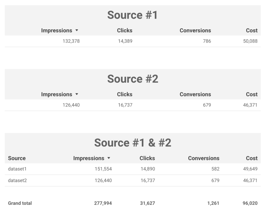
Here is a simple guide on how to merge data from various sources in Google Sheets. Let’s say you have two data source, for example, Facebook Ads and Google Ads, and that you want to sum their Impressions, Clicks, Conversions, and Cost. Here is a simple illustration made with Google Data Studio of what you will be able to achieve by following this guide.
[caption id=“attachment_1524” align=“aligncenter” width=“616”] Google Data Studio Dashboard with individual and merged data sets[/caption]
1. Organize your spreadsheet
The first important thing is to being organized. You won’t achieve anything if you are not able to properly structure and organized the data you want to merge. You will want to have a sheet for each source. You can have how many sources/sheets as you wish. Then You will want to have a master sheet where we will merge all your data source.
[caption id=“attachment_1525” align=“aligncenter” width=“597”] Google Spreadsheet architecture[/caption]
Your spreadsheet should look like this. For example, Source #1 would be Facebook ads data and Source #2 would be Google Ads data.
2. Apply the same template for each sheet
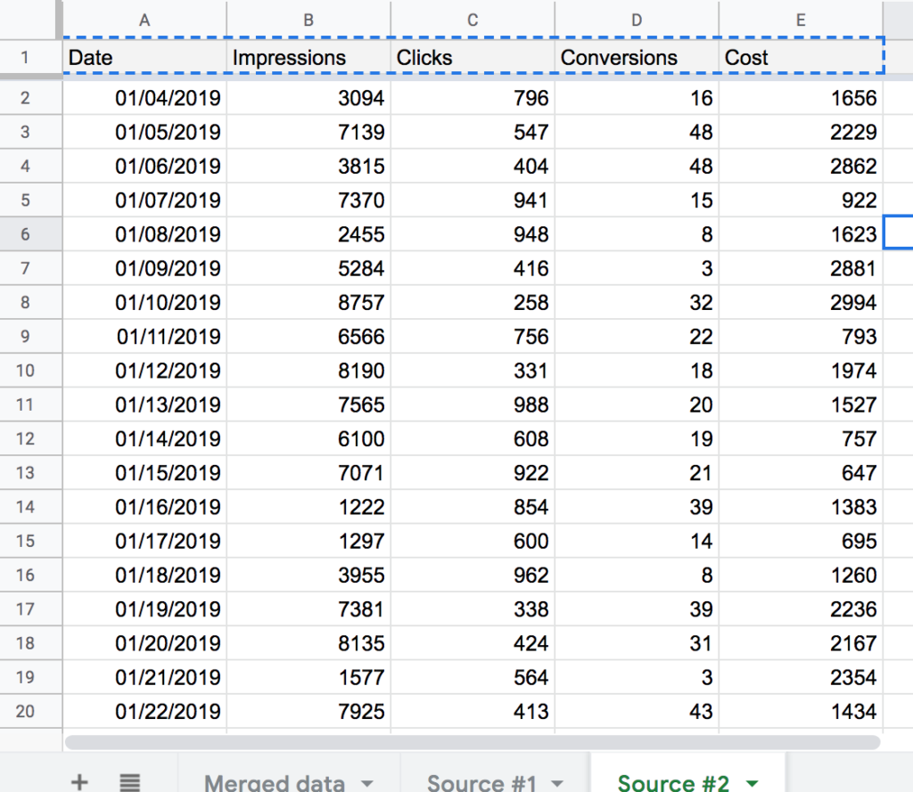
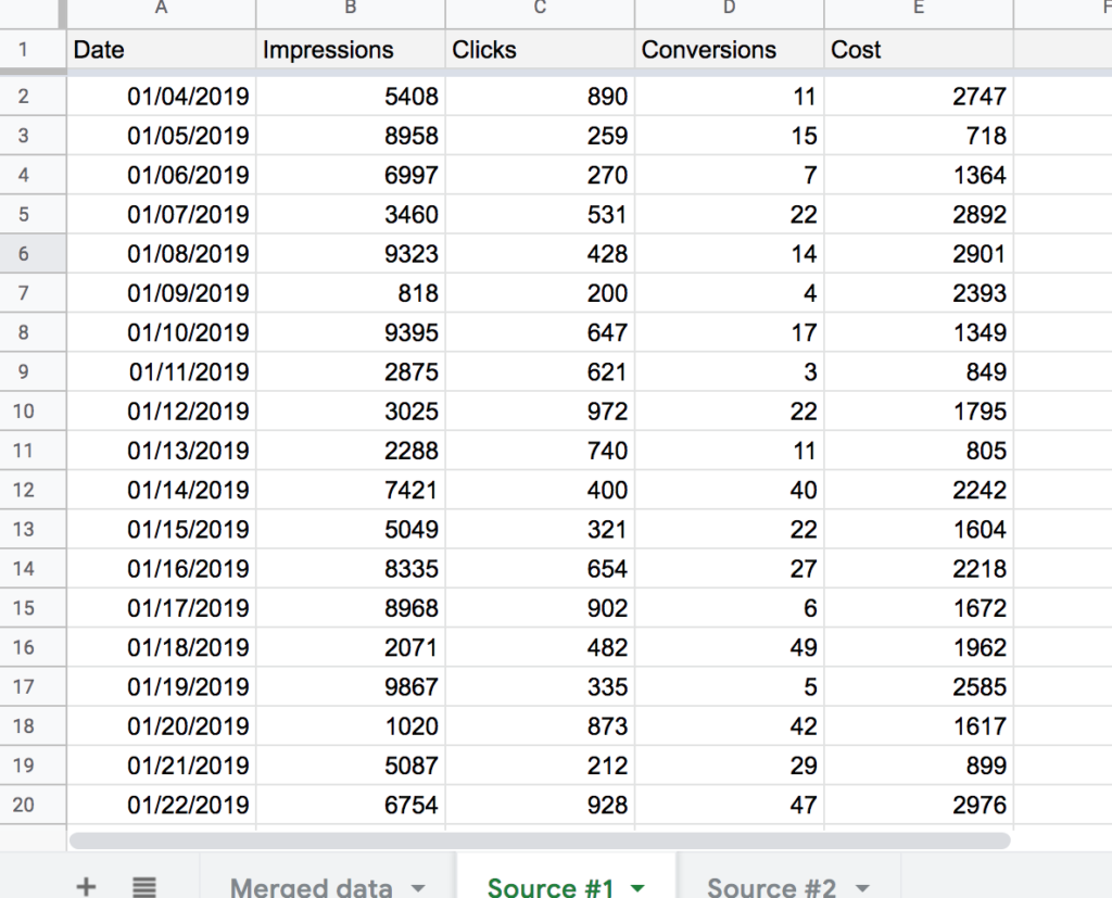
Each sheet will look likes the same. It is imperative to understand that if you want to merge various data set with the formula I will give you, you will need to have the same numbers of columns for each source (or you will need to tweak the formula). If you want to merge Google ads and Facebook Ads data, you will need to have, for example, Date, Impressions, Clicks, Conversions, Cost for each source in each sheet in the same order.
[caption id=“attachment_1526” align=“aligncenter” width=“304”] Source #2. For example Google ads[/caption]
[caption id=“attachment_1527” align=“aligncenter” width=“329”] Source #1. For example Facebook Ads[/caption]
3. “Merge data” sheet and formulas
This is where all the magic happen. The Merge data sheet will be organized the same way the other sources sheets (which mean five columns with Date, Impressions, Clicks, Conversions Cost in the same order) But instead of having data we will have one formula that will collect data from the source sheet and merge them into one data set. Here is the formula:
\=query(arrayformula({‘Source #1’!A2:E,iferror(‘Source #1’!A2:A/0, “dataset1”);‘Source #2’!A2:E,iferror(‘Source #2’!A2:A/0, “dataset2”)}), “select * where Col1 IS NOT NULL”)
The formula is querying each source sheet, looking for each row, adding one data set one after another. To more easily understand this formula it is possible to break it down in three parts:
The query
query(SOURCE, “select * where Col1 IS NOT NULL”)
With the query function, we are selecting all the row that are not null from our SOURCE.
The array formula part (SOURCE)
arrayformula({RANGE1;RANG2;etc…})
The array formula allows us to collect data from the various sheet as Range.
Range from each source
‘Source #n’!A2:E,iferror(‘Source #n’!A2:A/0, “datasetn”)
The error formula is a small trick allowing us to attribute for each row in the master sheet the name of the sheet from which it has been exported.
You can access the spreadsheet here and take a look at the formula and the spreadsheet architecture:
https://docs.google.com/spreadsheets/d/12iAPsWQfbS_ufMmCxEcFdUkRh_CBIJxHb0yDJW38HSg/edit?usp=sharing
Final thoughts
This solution works pretty well with Supermetrics on one side and Google Data Studio on the other side. With Supermetrics, you can easily automate the data collection of many sources. With Google Data Studio you can easily visualize the whole by connecting your dashboard to merge datasheet. This solution is flexible, low cost, and low tech.